Distributed ML

Contact me

• Blog -> https://cugtyt.github.io/blog/index
• Email -> cugtyt@qq.com
• GitHub -> Cugtyt@GitHub

---

来自Berkeley CS120x课程第二周Distributed ML。

Computation and Storage

Least Squares Regression: Learn mapping(W) from features to labels that minimizes residual sum of squares:

\[\min_W \Vert XW-y\Vert_2^2\]

Closed form solution, (if inverse exists):

\[W=(X^TX)^{-1}X^Ty\]

Consider number of arithmetic operations ( +, −, ×, / ), computational bottlenecks:

• Matrix multiply of $X^TX$: $O(nd^2)$ operations
• Matrix inverse: $O(d^3)$ operations

Consider storing values as floats (8 bytes), storage bottlenecks:

• $X^TX$ and its inverse: $O(d^2)$ floats
• $X$: $O(nd)$ floats

Computation: $O(nd^2 + d^3)$ operations

Storage: $O(nd + d^2)$ floats

Big n and Small d

Assume $O(d^3)$ computation and $O(d^2)$ storage feasible on single machine, storing $X$ and computing $X^TX$ are the bottlenecks.

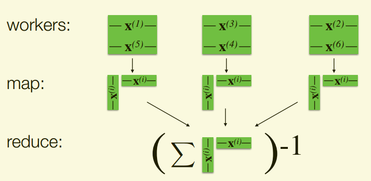
Can distribute storage and computation!

• Store data points (rows of $X$) across machines
• Compute $X^TX$ as a sum of outer products X

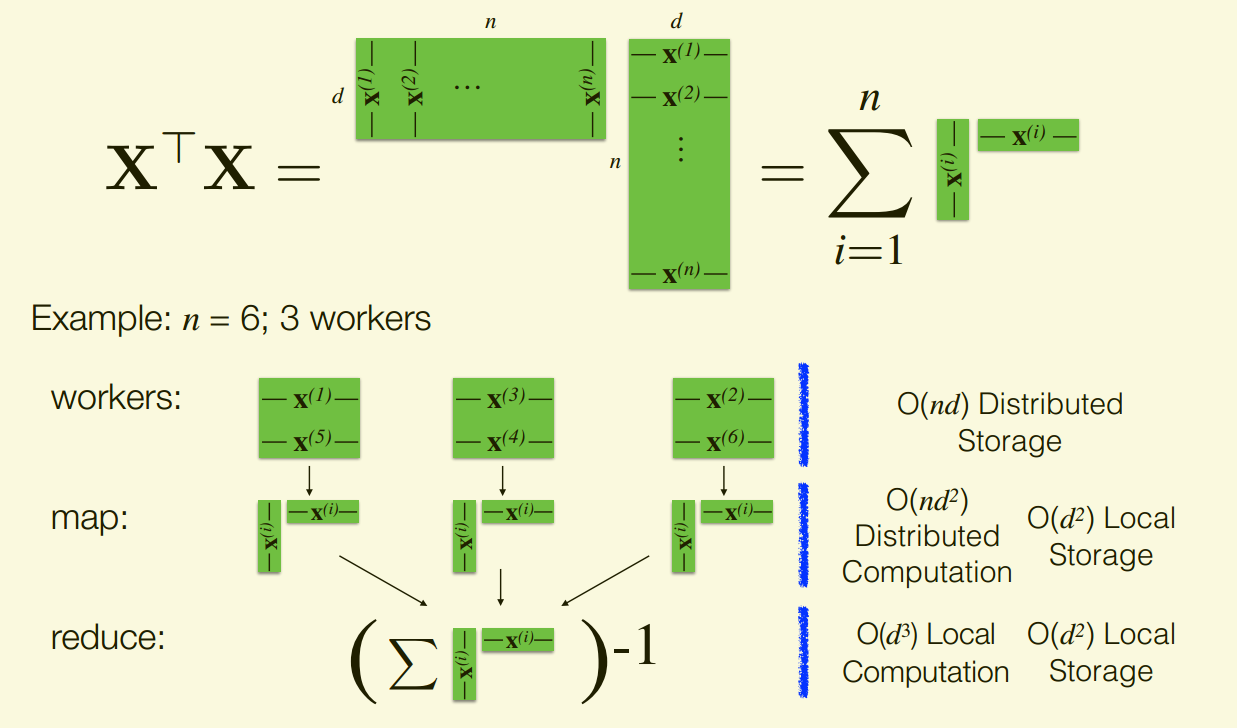
trainData.map(computeOuterProduct)         .reduce(sumAndInvert)

Big n and Big d

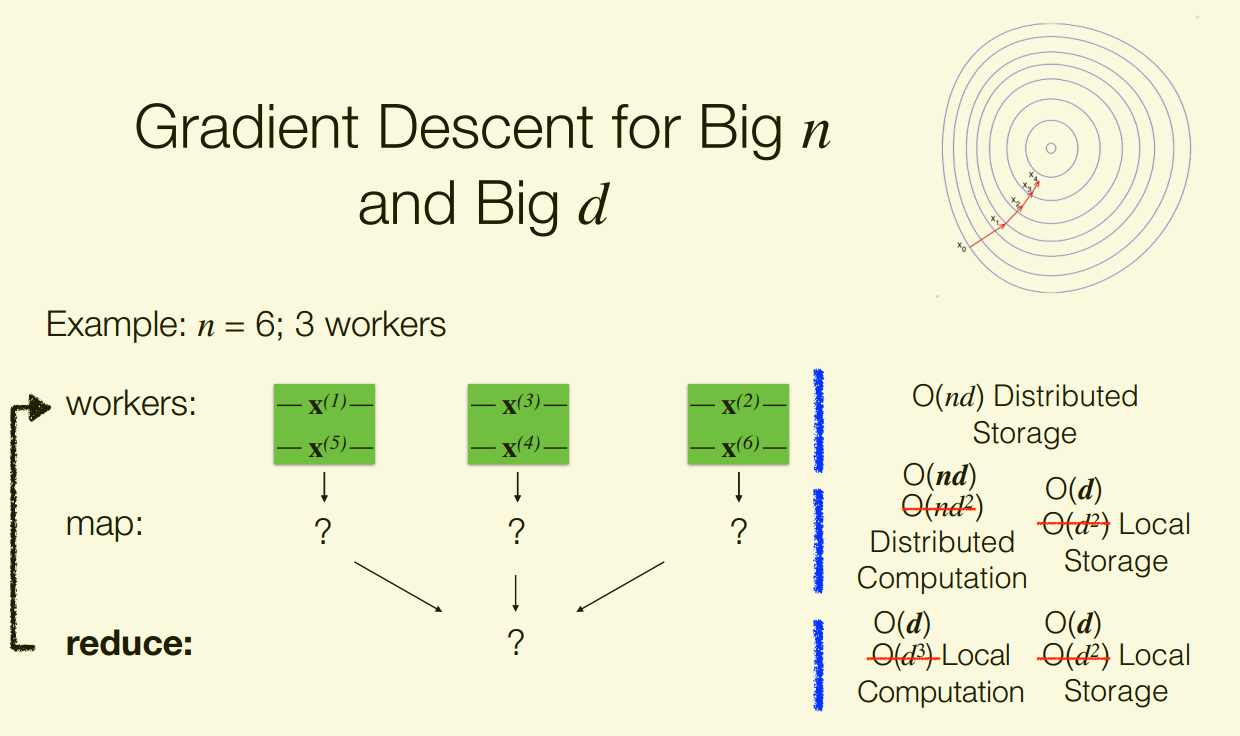
As before, storing and computing are bottlenecks Now, storing and operating on is also a bottleneck.

Can’t easily distribute!

1st Rules of thumb

Computation and storage should be linear (in n, d)

We need methods that are linear in time and space.

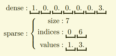
One idea: Exploit sparsity

• Explicit sparsity can provide orders of magnitude storage and computational gains

  Sparse data is prevalent:

  • Text processing: bag-of-words, n-grams
  • Collaborative filtering: ratings matrix
  • Graphs: adjacency matrix
  • Categorical features: one-hot-encoding
  • Genomics: SNPs, variant calling

  

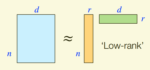
• Latent sparsity assumption can be used to reduce dimension, e.g., PCA, low-rank approximation (unsupervised learning).

  

Another idea: Use different algorithms

Gradient descent is an iterative algorithm that requires O(nd) computation and O(d) local storage per iteration.

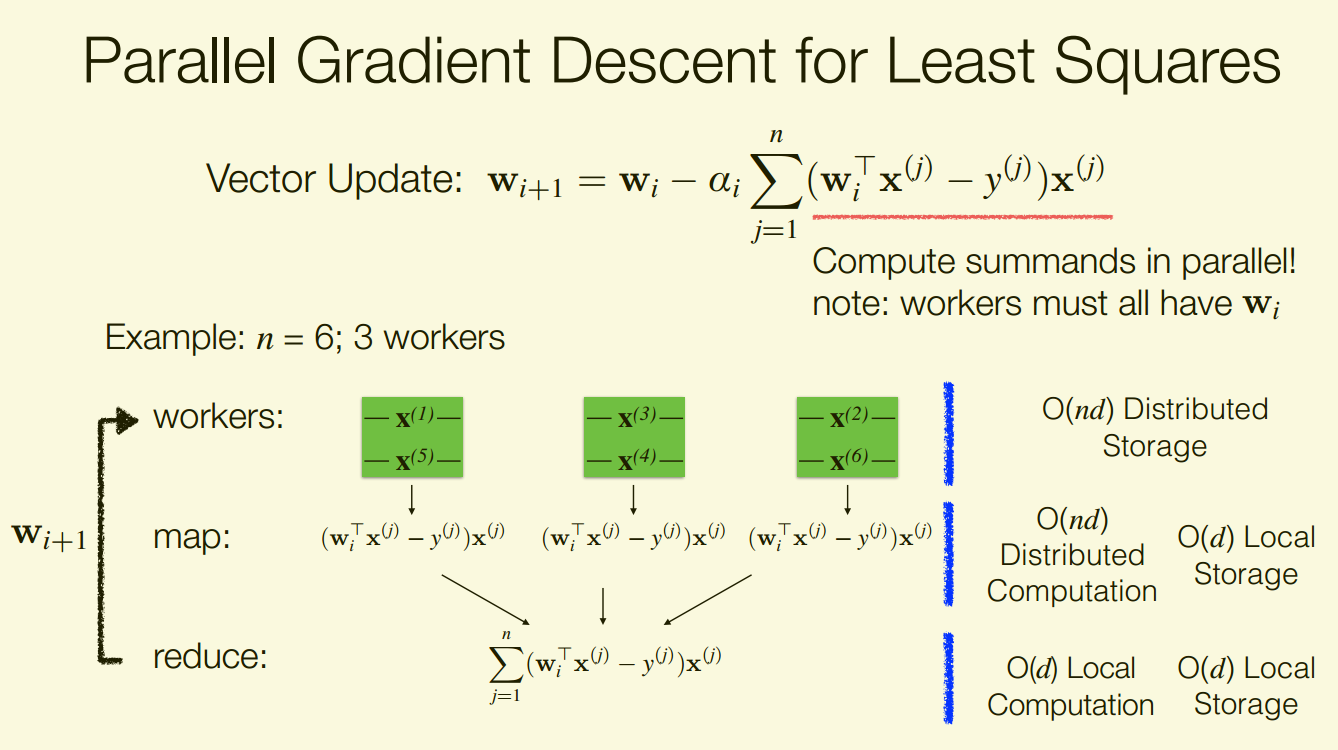
for i in range(numIters):
    alpha_i = alpha / (n * np.sqrt(i + 1))
    gradient = train.map(lambda lp: gradientSummand(w, lp))
    w -= alpha_i * gradient
return w

Gradient Descent Summary:

• Pros:
  • Easily parallelized
  • Cheap at each iteration
  • Stochastic variants can make things even cheaper
• Cons:
  • Slow convergence (especially compared with closed-form)
  • Requires communication across nodes!

Communication Principles

Access rates fall sharply with distance:

• Parallelism makes computation fast
• Network makes communication slow

2nd Rule of thumb

Perform parallel and in-memory computation

Persisting in memory reduces communication

• Especially for iterative computation (gradient descent)

Scale-up (powerful multicore machine)

• No network communication

• Expensive hardware, eventually hit a wall

  

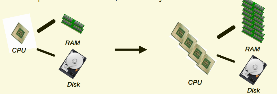
Scale-out (distributed, e.g., cloud-based)

• Need to deal with network communication

• Commodity hardware, scales to massive problems

  

3rd Rule of thumb

Minimize Network Communication

Minimize Network Communication - Stay Local

Example: Linear regression, big n and small d

• Solve via closed form (not iterative!)
• Communicate O(d2) intermediate data

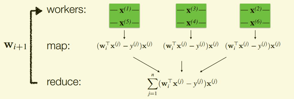
Example: Linear regression, big n and big d

• Gradient descent, communicate
• O(d) communication OK for fairly large d
• Compute locally on data (Data Parallel)

Example: Hyperparameter tuning for ridge regression with small n and small d

• Data is small, so can communicate it
• ‘Model’ is collection of regression models corresponding to different hyperparameters
• Train each model locally (Model Parallel)

Example: Linear regression, big n and huge d

• Gradient descent
• O(d) communication slow with hundreds of millions parameters
• Distribute data and model (Data and Model Parallel)
• Often rely on sparsity to reduce communication

Minimize Network Communication - Reduce Iterations

Distributed iterative algorithms must compute and communicate

• In Bulk Synchronous Parallel (BSP) systems, e.g., Apache Spark, we strictly alternate between the two

Distributed Computing Properties

• Parallelism makes computation fast
• Network makes communication slow

Idea: Design algorithms that compute more, communicate less

• Do more computation at each iteration
• Reduce total number of iterations

Extreme: Divide-and-conquer

• Fully process each partition locally, communicate final result
• Single iteration; minimal communication
• Approximate results

w = train.mapPartitions(localLinearRegression).reduce(combineLocalRegressionResults)

for i in range(numIters):
    alpha_i = alpha / (n * np.sqrt(i + 1))
    gradient = train.map(lambda lp: gradientSummand(w, lp)).sum()
    w -= alpha_i * gradient

Less extreme: Mini-batch

• Do more work locally than gradient descent before communicating
• Exact solution, but diminishing returns with larger batch sizes

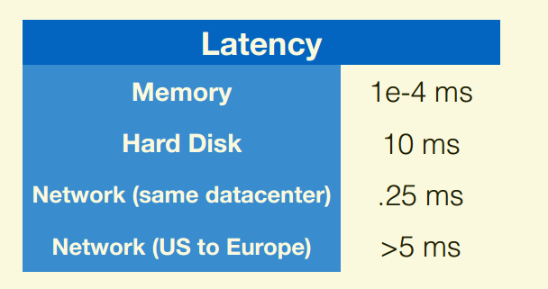
We can amortize latency!

• Send larger messages
• Batch their communication
• E.g., Train multiple models together

---

1st Rules of thumb

Computation and storage should be linear (in n, d)

2nd Rule of thumb

Perform parallel and in-memory computation

3rd Rule of thumb

Minimize Network Communication

---